First steps with Amazon Redshift

At Zemanta we have been using Amazon Redshift as our database of choice for campaign traffic statistics. We strive to deliver query results for our analytics view to our users close to real-time. This view is one of the core screens that our users use to manage their campaigns and see how well they perform, so it needs to be in shape.

Amazon Redshift is a great piece of technology but it does not magically produce good results. In fact, performance between an ad-hoc design and an optimized one can differ greatly. Table design and queries that you want to execute need to be tailored to how its internals work best and nourished along the way, when new features get developed and data grows in size. Only then we can get satisfactory results.

In this article we try to sum up the basics of efficient Amazon Redshift table design, and provide some resources that got us going in the right direction.

The basics

Amazon Redshift is a managed data warehousing solution whose main promise is that it can offer fast analytical queries on big data through extensive use of parallelism. It can load and unload big chunks of data directly from or to Amazon S3 (or other AWS storages) with which it integrates seamlessly. This is a big plus if your infrastructure resides in the AWS cloud as ours does. It can effectively do large data transformations and so can be used for your ELT (Extract, load, transform) pipeline. This is a great article from Panoply that compares ELT and ETL - the more common way of transforming data before loading it.

One of the common first impressions is that it’s actually some kind of PostgreSQL database because you can communicate with it with tools that are made for PostgreSQL, e.g. psql. It actually emerged from it, but as we will see, it is really far from it and should be treated differently.

Cluster

When you start using Redshift, you provision a cluster. A cluster consists of a leader node and multiple compute nodes. These are further subdivided into slices.

The leader receives queries, optimizes them, creates query plans and coordinates the work amongst its nodes. A node provides CPU, memory and disk for query execution and data storage. Memory and storage are proportionally allocated to its slices. A slice executes a single query segment within one process at a time.

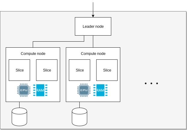Amazon Redshift cluster arhitecture.

More on cluster arhitecture and query execution workflow can be found in the official documentation here and here.

Data storage

The way data is stored and organized within a cluster directly influences how tables and queries should be designed for them to be performant.

The four most important concepts of data organization are: data distribution, sort keys, zone maps and compression. Here we will cover them briefly and provide some additional resources where you can research them in more depth.

Distribution

Distribution determines how data is distributed among slices. With it we define by what strategy should records be grouped together. By that we put data where it needs to be beforehand and so reduce the need for query optimizer to move data between nodes to efficiently query it. This comes in handy when we join data.

In the following example of data distribution we see traffic and conversion records grouped by campaign. When we join such data by campaign, no records need to be redistributed between nodes as they can be joined within a single slice. If distribution would be different and we would want to make the same join, records would need to be relocated temporarily before a query would execute.

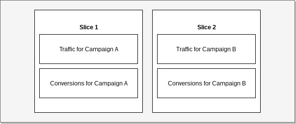Example: Data collocation.

With a proper distribution strategy we also try to evenly load nodes so that parallel processes have similar amount of work to do. The end processing time is determined by the slowest process. A node that has disproportionate amount of work to do, will thus directly influence the overall query execution time.

The consequence of uneven data grouping is skew (Skewed table data). In such cases some slices contain more data than others and can therefore slow our queries and cause premature fill up of storage on some nodes.

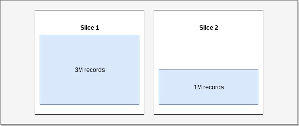Example: Skew.

Sort keys and zone maps

Redshift stores data in columns. This means that blocks of values from the same column are stored on disk sequentially as opposed to row based systems where values from a row follow sequentially.

Sequential values of a column are partitioned within 1MB blocks that represent the smallest data organizational unit. Redshift will load an entire block to fetch a value from it, so it is important for us to understand how it decides to select a block. This way we can minimize I/O operations.

Sort keys set the order of records within blocks and tables. It behaves the same as ORDER BY in queries.

Zone maps are meta data about blocks, they define MIN and MAX value within them. Using sort key and zone map information Redshift can skip blocks that are irrelevant for a particular query.

In the following example we will try to illustrate the difference in the amount of I/O required to locate the offset of relevant records. We defined a table that has clicks grouped by date and campaign id. We have ordered the data by date. To query clicks by campaign for the date 2017/02/12, Redshift will be able to find relevant records by loading and reading only the 1st date column block. On the other hand, when we would like to get clicks for campaign id 500, 2 blocks will have to be loaded and read to get the record offset for other columns.

CREATE TABLE stats (
    date date not null,
    campaign_id int2 encode lzo,
    clicks integer encode lzo
) sortkey(date)

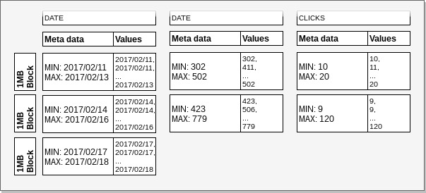Example: Sort keys and zone maps.

When adding data to our tables we need to maintain the sort and meta data. We can either add data in correct order or we can use VACUUM to resort and ANALYZE to update meta data and table statistics.

Compression

Due to Redshifts columnar nature it can efficiently compresses the data it holds. This means that the amount of data within a 1MB block can be increased and the overall storage footprint reduced. This can save us some I/O because less data needs to be read from a disk. Because it is columnar it can also independently of other columns shrink or grow records within one column.

In the Sort keys and zone maps example we can see different storage requirements for the date and campaign id columns. We see that the same amount of values for dates took 3 blocks, and only 2 blocks for campaign ids. This happened because the compression of the campaign column was better.

By default no compression is applied to data. A good first start is the command ANALYZE COMPRESSION that we execute on already loaded data and it will give us recommended encodings based on a sample. If we have some knowledge about our data we can also select encodings ourselves. Available algorithms and when to use them are listed here.

Code compilation

Not related to the way data is stored but important concept used by Amazon Redshift is code compilation.

When Redshift receives a query, it will optimize it and generate a query plan. Execution engine will take that query plan and generate compiled C++ code from it. After that it will put it into a LRU cache. The compilation step can take a while and this is why you will notice that the 1st run of a query is always, sometimes by an order of magnitude, slower than the following runs of the same query. Later runs of the same (or similar) query will take the compiled code from cache and thus the compilation step will be skipped.

A query won’t need to be recompiled if only some filter parameters get changed. On the other hand, Redshift will recompile a query if everything is the same but different or additional columns are selected. Unfortunatelly not much is documented about what changes have an effect on recompilation. In this article the author tries to experiment a bit and find some patterns.

Cases when we need to be aware of this behaviour are benchmarks and dynamic query building. When we do benchmarks we always ditch the first query execution time as it will always be an outlier. Where we do dynamic query building we try to reduce the number of unique queries. One way we do that is that we always query all columns that are available for a given view. We strip the ones that we won’t show later, e.g. based on a permission. This way a query for the same view but two users with different permissions will be the same or similar enough that it won’t need to be recompiled.

Conclusion

We have been using Amazon Redshift for more than a year now and we are pretty comfortable with it by now. We think the concepts described in this article will give you a good start with fundamentals of optimal table design that are needed for a beginner in this field.

We realize there is a lot more to it, so we selected a few more resources that helped us, and we are sure will help you, on going further and deeper on it in the last chapter Additional resources of this article.

Additional resources

• Top 10 Performance Tuning Techniques for Amazon Redshift
• Improving Redshift Query Performance Through Effective Use of Zone Maps
• The Lazy Analyst’s Guide to Amazon Redshift
• The Hitchhiker’s Guide to Redshift 
• Amazon Redshift Deep Dive
• Deep Dive: Amazon Redshift for Big Data Analytics (video)
• Redshift at Lightspeed: How to continuously optimize and modify Redshift schemas
• Amazon Redshift - Database Developer Guide (official documentation)

Keeping Secrets in Plain Sight

What is a secret? It’s information we don’t want others to know. In the context of server side applications the secrets are database passwords, API tokens, private keys and other information that we want to keep secret.

Many of such secrets are specified in the configuration files, alongside items that don’t necessarily need to be secret, such as database names, debug flags and other configuration.

As a result, production configuration files are often kept encrypted in a separate repository then decrypted at deploy time. This approach works, but becomes cumbersome when the non-secret configuration is frequently changed or when new secrets are often added to the application. Because every change to the configuration involves re-encrypting the file, we need to deal with both a separate workflow for these changes and losing the ability to git blame individual configuration properties.

At Zemanta, we wanted a way of managing secrets that would enable us to:

• add a new secret to an application in a straightforward and simple manner,
• enable quick and simple configuration changes,
• update a secret and still be able to inspect previous versions,
• attribute a secret to an application,
• use one pattern to manage secrets across all of our applications.

SecretCrypt

To address the above points, we created SecretCrypt, a tool for keeping encrypted secrets inside configuration files that reside in the app’s codebase (and by extension in its code versioning system of choice like Git). The secrets are then decrypted on the fly when the application is started.

For example, a Django settings.py file containing secrets looks something like this:

from secretcrypt import Secret

# the encrypted secret
GOOGLE_OAUTH_CLIENT_SECRET = Secret('kms:region=us-east-1:CiDdfiP9DHF5...rQG/YJrGQ==').get()

# other, non-secret configuration
GOOGLE_OAUTH_ENABLED = True
GOOGLE_OAUTH_CLIENT_ID = '22398899238-123ji2o1i4u2198042jio.apps.googleusercontent.com'

Since the configuration file is kept in the same repository as the code, configuration options or secrets can easily be changed or added by developers themselves. We also get the history of all the changes as an extra feature, since secrets are subjected to version control and the encryption is performed per-secret, not per-file.

How it works

To achieve this, we make use of AWS’s Key Management Service (KMS). KMS allows us to create encryption keys that can then be used with the service’s encrypt and decrypt endpoints. Permissions to encrypt or decrypt something with a given key are mandated by IAM policies. In our case, we’ve set up key permissions in such a way that our developers have the permission to encrypt new secrets, but cannot decrypt them. On the other hand, the EC2 instances that run the application are assigned an IAM role that has the permission to decrypt those secrets.

Alternative secret backends

SecretCrypt is designed in a modular fashion, so it can support multiple encryption/decryption backends. Alongside KMS it currently also supports local encryption, which uses locally generated keys for AES encryption and is intended for local development purposes.

An alternative to the KMS backend could also be HashiCorp’s Vault, which is a self-hosted encryption-as-a-service (among other things).

Adding a new secret

A new secret can be encrypted using a CLI tool by simply passing the alias of our KMS encryption key:

$ encrypt-secret kms alias/Z1secrets
Enter plaintext: VerySecretValue!
kms:region=us-east-1:CiC/SXeuXDGR...

and then included in the Python file as

from secretcrypt import Secret

MY_SECRET = Secret('kms:region=us-east-1:CiC/SXeuXDGR...').get()

When the Python file is loaded, SecretCrypt will use KMS to decrypt the secret. It uses boto, so it supports AWS credentials from various sources, such as local configuration, environment variables, EC2 roles, etc. (view more)

Go version

Since we wanted to use a single secrets workflow for all our applications, we also developed SecretCrypt for Go. It implements the TextUnmarshaler interface, so it supports various configuration file formats such as TOML,

MySecret = "kms:region=us-east-1:CiC/SXeuXDGRADRIjc0qcE...

YAML,

mysecret: kms:region=us-east-1:CiC/SXeuXDGRADRIjc0qcE...

or JSON.

{"MySecret": "kms:region=us-east-1:CiC/SXeuXDGRADRIjc0qcE..."}

The secret is then used in the application’s config struct:

type Config struct {
    MySecret secretcrypt.Secret
}

var conf Config
if _, err := toml.Decode(tomlData, &conf); err != nil {
    // handle error
}
plaintext := conf.MySecret.Get()

Conclusion

In the end, developer tooling is all about reducing friction. SecretCrypt has allowed our developers to tweak configuration in production without having to re-encrypt the secrets. It has also enabled them to add new secrets without the assistance of the ops team. We are now able to track the history of the changes of both our configuration and our secrets.

We have been using SecretCrypt in production for almost six months now! We were able to drop a separate encrypted Git repository and the corresponding workflow that we used for configuration previously. Simply change, commit, and deploy!

Discuss on Hacker News

Guide to Engineering at Zemanta

At Zemanta we believe in writing things down — i.e. if it’s not in writing it doesn’t exist. We take notes on every single meeting in google docs, we write down our product ideas and turn those notes into product requirement documents, we write down technical requirements on new systems we’re about to design or redesign existing ones, we document our product feature roadmaps so everybody knows what our goals are … and we’re not the only one in the tech space with such beliefs.

Why? Keeping people in sync. We have a large group of people working on a single product and keeping a multidisciplinary group of engineers, data scientists, product managers, sales people and marketers that are spanned across 2 continents in sync, can be profoundly difficult.

How does writing it down help keeping people on the same page? Think how many times did you lead/attend a meeting, where everything was clear to everybody, but 2 days later, people started making wrong assumptions and conclusions about what was agreed upon. Sounds familiar? There’s nothing wrong with that and it’s human nature you’re fighting against. Psychologists who are researching the effectiveness of eye-witness testimony in courts, say that people don’t have video recorders built in their brain and they can’t just play back the meeting, but instead, have to “reconstruct to remember”.

Keeping things in writing, allows people to meet, debate, write down the consensus, think about the the conclusions in private and follow up, if they require more clarification.

Documenting our engineering culture, tooling and process is no exception to the principle of writing things down. Not having a very basic written outline of our engineering process and practices, turned out to be very painful for new hires that joined a team that was well in sync for the last 2 years. There were a lot of intricacies, tools and non verbal expectations to our process that was very confusing to somebody just joining our team.

After noticing this confusion we decided to write a guide to engineering at Zemanta from a perspective of a new technical hire that would serve as a brief guide to tools, practices, process and principles of coding and some parts of the operations. We’re emphasizing the word brief guide, since there are still a lot of intricacies left out, but it’s good enough for getting around confidently on the first days at work and getting that first pull request onto production.

github.com/Zemanta/engineering-at-zemanta

We decided to put this guide on github because of:

1. every engineer in the company can propose changes to the process and practices by opening up an issue or a pull request with proposed changes, that are then subject to discussion and consensus

2. putting it on github keeps it close to code and in sight — if we would just put it in a doc on google drive the whole guide would quickly become out of sight and out of mind

3. inspired by our colleges at Lyst, we also decided to open source the guide — there’s open source software, why not have an open source guide to engineering

In conclusion, we recommend a practice of documenting every process (or as much as possible) in your company and maybe our guide can give you a head start — feel free to fork it and adapt it to your needs.

Railway to Craftsmanship

Maybe “highway” would be more appropriate, since I didn’t take the train to get there. But even so, the pervasive theme of the Craft Conference 2016, which took place between 26th and 29th of April in the beautiful Hungarian capital of Budapest, were trains.

The event took place at the picturesque Magyar Vasúttörténeti Park (Hungarian Railway History Park), which is exactly what you think it is — a big park filled with over a hundred old trains. As you can imagine, it makes for quite a unique conference venue. How to get there, you ask? Hop on the Craft Train, an actual train that takes you from the centrally-located Nyugati Terminal to the venue and back, twice a day. So, rail-heaven.

Notice the train.

The conference delivered on other aspects as well (which is especially important for people who are not fanatical about trains). It was well organized, with all the important info sent to us well in advance. For the duration of the conference (i.e. two workshop days and two conference days) the participants were taken good care of with catered breakfasts, lunches and even dinner on some days. Being bored in the evenings was not an option — there were more than 10 meetups on various tech topics, ranging from Docker, agile to functional programming. All these were taking place after the conference schedule ended for the day, followed by a common afterparty at the Google Ground.

But of course, the most important question is: “How was the speaker lineup?”

Speakers

When you hear that the event was taking place somewhere in eastern Europe and not in a western city like London, Paris or Berlin, you just might think that this comes at a cost of a “lesser” speaker lineup. You are so wrong!

The lineup was instead rather impressive — featuring speakers like John Allspaw, Martin Fowler, Marty Cagan and Michael Feathers, to name just a few. Major players in tech space were well covered too — there was no shortage of speakers from companies like Twitter, Uber, Google, Docker and Stripe. Another great fact — 25% of speakers were women. This is quite amazing for such a hardcore dev conference (could be even better of course).

The format of the conference was fairly standard. The first two days were full-day workshops in different locations across Budapest — 11 workshops per day. Followed up with two regular conference days.

Instead of walking you through all the talks I’ve seen, I’ll present the three main topics instead.

Microservices

If I would describe the whole event in one word, it would be “microservices”. If I could use three, it would be “microservices absolutely everywhere”. Microservices seem to be the hottest buzzword at this moment. So of course I attended a lot of these talks to see what all the fuss is about.

Actually, my whole first half of the conference was about microservices because of my workshop selection. The first one, titled simply “Microservices”, was presented by Adrian Cockcroft. “Who is he and why does he think he knows anything about this topic?” Well, Adrian is most well-known for his time at Netflix, where he led the company’s transition to a large-scale, highly-available public-cloud architecture, based on a large number of small services. That was back in the time when Docker and all the modern tools had yet to materialize, so you could think of him as one of the pioneers of the microservices architecture.

Then there was the other workshop by Sam Newman, titled “Building microservices”. Sam works at Thoughtworks and is well known for his recent book Building Microservices. During the workshop, he appeared to be a fun guy with substantial experience on everything about the topic — the workshop itself was half listening to his presentation about microservices and the issues that arise when trying to implement them and half hands-on session with the materials which he shared with us on a USB stick. All this was followed by a long Q&A session where we discussed various topics that were not covered in the material.

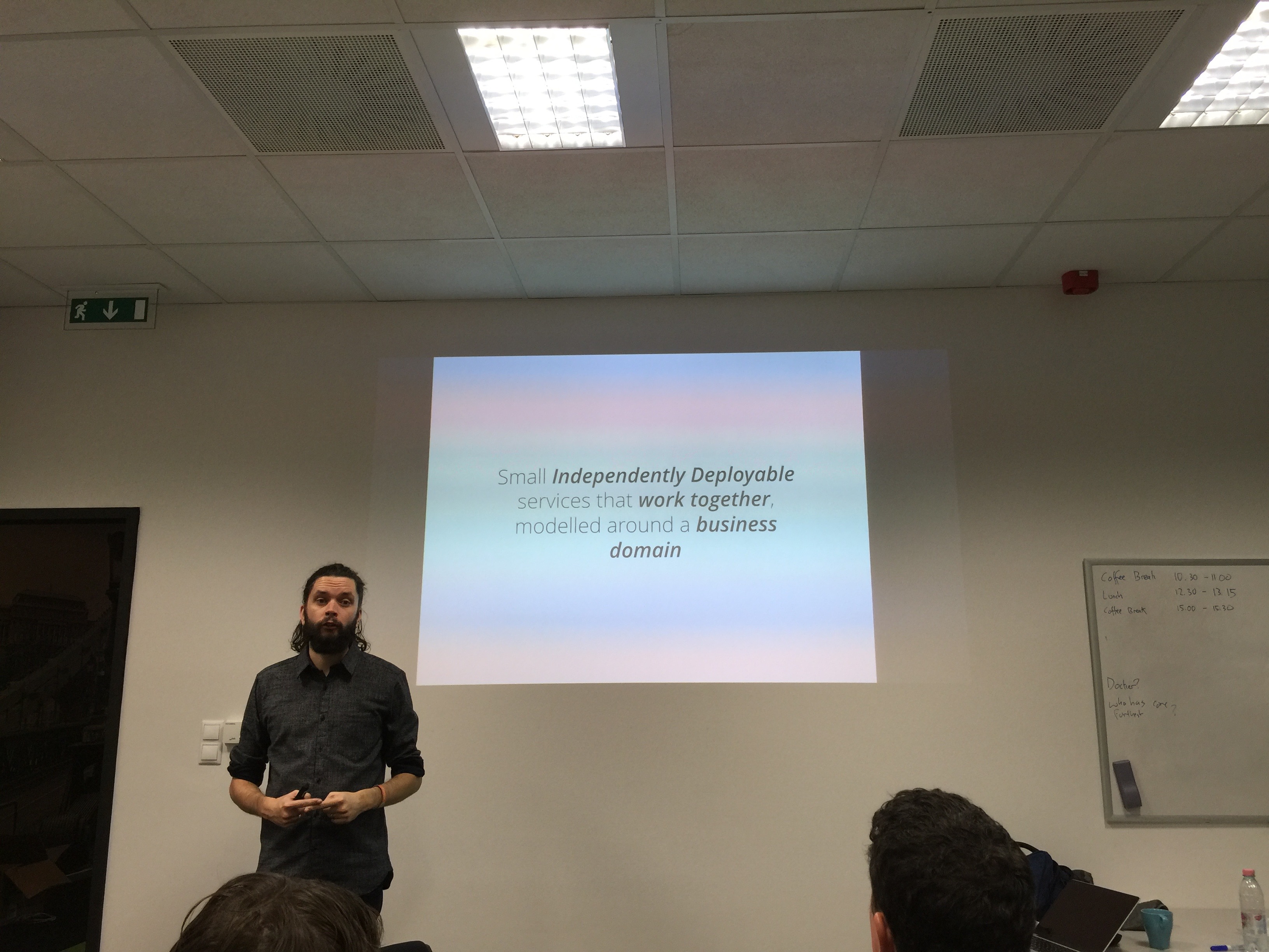Sam Newman on microservices.

So what about microservices? What are they really? Both workshops gave a slightly different definition. Cockcroft suggested that they are “a loosely coupled service-oriented architecture with bounded contexts”, while Newman’s definition was “small independently deployable services that work together, modeled around a business domain”. Give it some thought and you’ll realize that, both are quite similar. The main takeaway is that all components are independent — i.e. if you have a group of services which you always need to deploy exactly at the same time or things will break, you’re not playing by the rules. The other implication is nicely illustrated by Conway’s law — which basically says that the architecture produced by the organization will reflect the communication structure of that organization.

These properties supposedly provide a nice advantage — in a large organization, individual teams can be more independent and can move much faster — there is never any need to wait for other teams. Each team works in its garden of microservices, uses whatever technology they feel will be the best fit and deploys them at their will. Each microservice also scales independently.

But of course, there are downsides. These can be summed up in just three words: increased operational complexity. For example, monitoring becomes more complex, as you need to monitor tens or even hundreds of services instead of just a few. Integration testing becomes a big pain. The communication between services gets quite complicated. What used to be a simple in-process function call is now made over the network, which is not nearly as reliable. Transactions are much harder in distributed systems. Fortunately, these are all solvable with modern tools. Both workshops gave a good overview of handling these sort of challenges .

Beyond microservices

Cockcroft also talked about his view of the future of microservices. As the trend continues, we will likely transition into what he called “serverless architecture” — an architecture where a unit of deployment is not a microservice, but just a function. An example of this are Amazon’s Lambda functions, which are configured on AWS. When such a function is called, a container is run just for the duration of the call and then shut down again. We explored this at another hands-on workshop by Danilo Poccia - an Amazon evangelist, where he showed how it is possible to build a whole backend for a mobile application by using just Lambdas and other AWS provided tools. Exciting!

Some other talks I attended were by Google’s Kelsey Hightower, demonstrating the use of gRPC and Kubernetes, Docker’s Jérôme Petazzoni showing how to use Docker Swarm in production, and Caitie McCaffrey from Twitter talking about building scalable stateful services. All were great and very informative - with a possible exception of Petazzoni’s talk, but that’s just because I am a Docker beginner and his talk was a bit too advanced for me.

FRP

Another well-represented topic was functional reactive programming, or FRP for short.

One of my favourite talks of the whole conference was Jessica Kerr’s talk about Elm. Elm is a relatively new programming language for building user interfaces, like web apps. Its creator, Evan Czaplicki, is quite an ambitious man — his aspiration is for Elm to be the next big thing in frontend development and to actually replace JavaScript. Sounds crazy? Maybe, but there’s no denying that Elm is an interesting little beast. It is a pure functional language with a very clean syntax (inspired by Haskell) and a strong type system. But fear not — one of its the main design principles is: ease of use. Easy to use, to the point, where developers with very little experience can make meaningful modifications to the code.

Evan Czaplicki as desktop background image.

Elm has very nice properties. For example, if your code compiles, it’s almost guaranteed to work and it will never ever throw a runtime error. Even though you wouldn’t expect it, since it compiles to javascript, it is very fast. It also introduces Elm architecture, which is a very simple pattern to be followed when building programs.

Mrs. Kerr was a great presenter, because of her huge enthusiasm for the language and she also produced a great tutorial.

Culture

Of course, there was no shortage of various culture/product/team organization talks. One of the most interesting, titled Architecture without Architects, was given by Martin Fowler and Erik Dörnenburg. They spoke about the role of architects in software development. They concluded, that they are not very useful. At least not in the traditional sense where an architect is someone who plans a whole software system up-front and hands it to engineers. They argued: while software architecture is usually compared to an actual, construction architecture’s job, it is instead more similar to town planning. The architect’s role should therefore be more about providing a good environment and guidance for engineers, which will ensure that the architecture evolves organically in the best possible way. Or, as Fowler put it: “The most important artifact of an architect are improved developers”.

Martin Fowler and Erik Dörnenburg explaining why real architects are not a good analogy.

Charity Majors also produced a great talk on the importance of operations skills for engineers. To build truly effective teams, engineers should have enough operational skills to be able to really own their services end-to-end, including deployment and monitoring. This doesn’t mean that dedicated operations engineers are not required anymore, but simply that developers shouldn’t be ignorant about these aspects. Not owning the mentioned skillset would slow the whole team down. We already expect operations engineers to know how to code and know at least the basics of technologies that will run on our infrastructure, so it should also be the other way around. Majors actually argues that any engineer who refuses to learn these skills should simply not be promoted until he does.

Product

Then there was the great Marty Cagan with a closing keynote on the first conference day. He spoke about what it takes for a team to make a great product. The talk was PACKED with great insights, but let me try to sum them up. A great product team will be composed of all roles: product, UX, engineers, operations etc. On top of those roles the team should be focused on business outcomes. That is, a team should not get a list of features that need to be built, but should instead be given high level objectives/problems, and be empowered to figure out how to solve them. As you can see, this plays nicely with the idea of microservices, where the core idea of team structure is very similar.

The other point Cagan made was the importance of fast discovery. It is considered to be a good practice for the team to function in two separate tracks — discovery (where ideas are validated in form of MVPs as quickly and cheaply as possible) and delivery (where features are actually built and delivered). The important distinction is, that discovery prototypes should be light i.e. not made by engineers, but built with various prototyping tools who don’t require engineering skills to master.

Conclusion

To be honest, when choosing a conference, I didn’t really think of Craft as of much of a contender. But after seeing the impressive list of workshops and talks, I decided to give it a shot. And let me tell you, it was definitely a good choice. Almost all talks I attended were good or even great, the event was very well-organised and quite unique. The entire event was not too commercialized while still having that grand impression of a first class international conference. I may stop at this station again in the future.

Why we migrated away from Librato to InfluxDB?

About 2 years ago we’ve jumpstarted our Native DSP platform. At the time we needed to move fast and think tactically. Making sure we make the most of our time every step of the way.

Setting up and managing the infrastructure for a metrics backend like Graphite was certainly not considered a priority at the time. So we started out with a managed metrics service and then migrated our metrics infrastructure to a modern open source stack.

Metric Types

Our application emits a ton of metrics of various types:

• Performance metrics - per request timers and counters, internal api call timers, …
• Application state metrics - e.g. number of items waiting for processing
• System level performance metrics - e.g. AWS CloudWatch data on RDS & SQS
• Composite metrics - metrics that are a function of other metrics i.e. if you have requests per second and number of cores in your autoscale cluster, you can observe requests per second per core

To manage all these metrics we require a metrics backend capable of ingesting measurements in real time and a flexible data visualization platform with a capability of displaying large number of metrics on standalone screens we have hanging on various parts of our office.

We consider New Relic as a great addition to the end solution, but not as a standalone-solve-it-all platform for our requirements.

Starting with Librato

At that time Librato offered a great shortcut to get up and running quickly without having to worry about any capacity planning, since librato offered that we simply pay everything “on demand”.

Below you can see the gist of our architecture with respect to our metrics backend (Librato) with major complexity abstracted away.

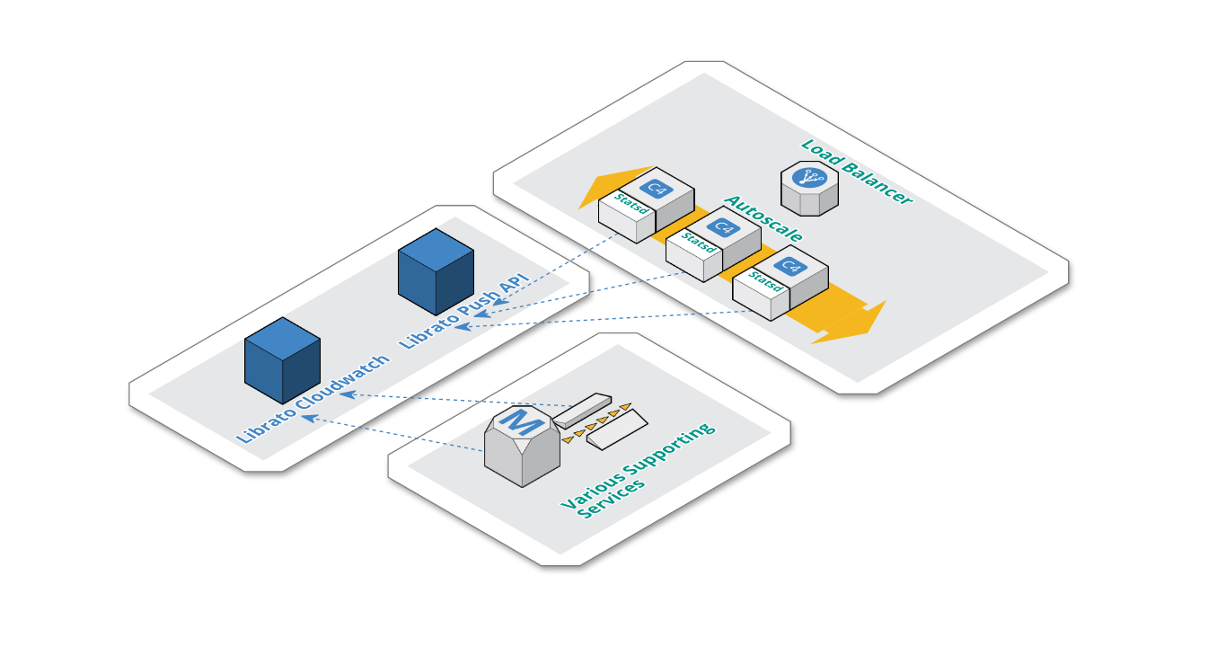
• Application nodes, which are autoscaled, each have an instance of Statsd. We’ve made this pragmatic design decision, because Statsd had a low resource footprint on each application node, thus eliminating the need for any highly available centralized Statsd setup.

• Statsd is configured with a librato backend and flushes metrics via librato push api every 10 seconds.

• Librato CloudWatch integration pulls metrics about supporting services (SQS, Redshift, RDS).

Librato Cons

Librato pricing can be a bit tricky and hard to wrap your head around, if you’re sending data to them from multiple sources (i.e. nodes) and those node’s unique identifiers are short lived (i.e. autoscale). The costs for such metric streams simply add up in your bill.

We also never fully understood how librato rolls up data. Their complexity around metric periods with respect to rolling up was not really a good fit for us. At times it was really frustrating setting up real time and long term trend dashboards that made sense for us.

Librato dashboard also has no mobile support. This feature turns out to be really important, if you get an infrastructure alert in the middle of the night and are not able to check your metrics from the comfort of your bed.

Librato Pros

Librato is a great pick, if you want to get your metrics backend up and running quickly, since it’s only a credit card away. If you only need to observe a small volume of metrics, then librato can be cost effective, since you pay everything on a per metric per frequency basis.

Librato also comes with a very basic alerting system. Providing you with basic means to set up alerts based on short term trends. Short term? Yes — Librato only allows you to observe a metric trend for 60 minutes and making a decision based on that time window.

A direct AWS CloudWatch integration is a great asset of Librato. You’re able to get all your metrics in a single platform very quickly and that was a great value for us.

You can start pushing in metrics in a manner of minutes. We suggest a statsd to librato integration since they have written a librato backend for statsd (fyi: If you’ll use our “battle tested” fork, you’ll have better support for extracting source names from your legacy metric names).

All in all Librato, is a great service with a few glitches that can outweigh the value of a managed and well supported platform.

Looking for Alternatives

Complexity and volume of our metrics started to grow and so did our interest of looking for better, more cost effective and easier to use metric platform.

We wanted to keep the good parts of our current platform, but we certainly wanted more control and transparency when compiling metrics into dashboards and more control when setting up alert conditions.

The options were:

• Self hosted Graphite + Grafana + Some alerting component (e.g. Cabot)
• Hostedgraphite.com
• OpenTSDB
• Prometheus.io
• Some parts of the TICK stack (Telegraf + InfluxDB + Chronograf + Kapacitor)

We quickly eliminated hosted Graphite since you pay per metric and since we’d like to have short lived server names in our metrics, we would quickly generate a lot of them. This solution wouldn’t be cost effective in the long run.

OpenTSDB seemed too heavyweight, since you need to manage an entire HBase cluster as a dependency.

Promoteheus didn’t seemed like a good fit since we prefer the metric push approach opposed to metric pull.

Self hosted Graphite was a viable option too, but the notion of being able to tag your metrics was a feature in favor of InfluxDB which was our final call.

Out of the box we identified that InfluxDB has no support for composite metrics, but the InfluxDB stack has a component that solves this problem for you (we’ll get to that later in the blogpost).

InfluxDB Killer Feature

I mentioned that InfluxDB by itself has a very appealing feature of being able to tag your metrics. In our case this proves to be exceptionally useful, since we’re building and monitoring a distributed real time bidding platform. We want to be able to take a very fundamental metric bid_throughput and then break it down by host and exchange in our example.

bid_throughput,host=server01,exchange=google    value=20 1437171724
bid_throughput,host=server01,exchange=yahoo     value=21 1437171724
bid_throughput,host=server02,exchange=outbrain  value=23 1437171724
bid_throughput,host=server02,exchange=adsnative value=20 1437171724

Tags in InfluxDB are indexed, which means querying series by tags is very fast. You can make the most use of that by storing data you want to break down by (e.g. you want to use them in GROUP BY) as tags.

On the other hand, tags being indexed means that you want to avoid storing high cardinality data such as random hashes in tags, since that will cause the size of your index to grow without bounds.

Transition to TIGK Stack

• T = Telegraf - replaced statsd as the agent that writes to InfluxDB
• I = InfluxDB itself
• G = Grafana - in our opinion a superiour tool to Cronograf at the moment
• K = Kapacitor - alerting and metric processing system

This stack was our final pick for our metrics platform.

Getting Data in

We use telegraf as a near drop in replacement for statsd. Telegraf has a compatibility layer with statsd with an extension that enables you to utilize InfluxDB tags.

Calls to telegraf are made by our django and go-lang apps directly, using the Zemanta/django-statsd-influx client. (We’ll be opensourcing our Go-lang client soon.)

We have metrics about our managed services (e.g. ELB, RDS, Redshift, SQS) that end up on AWS CloudFront being pushed via a cron scheduled AWS Lambda function. Admittedly, one of our best uses of AWS Lambda so far.

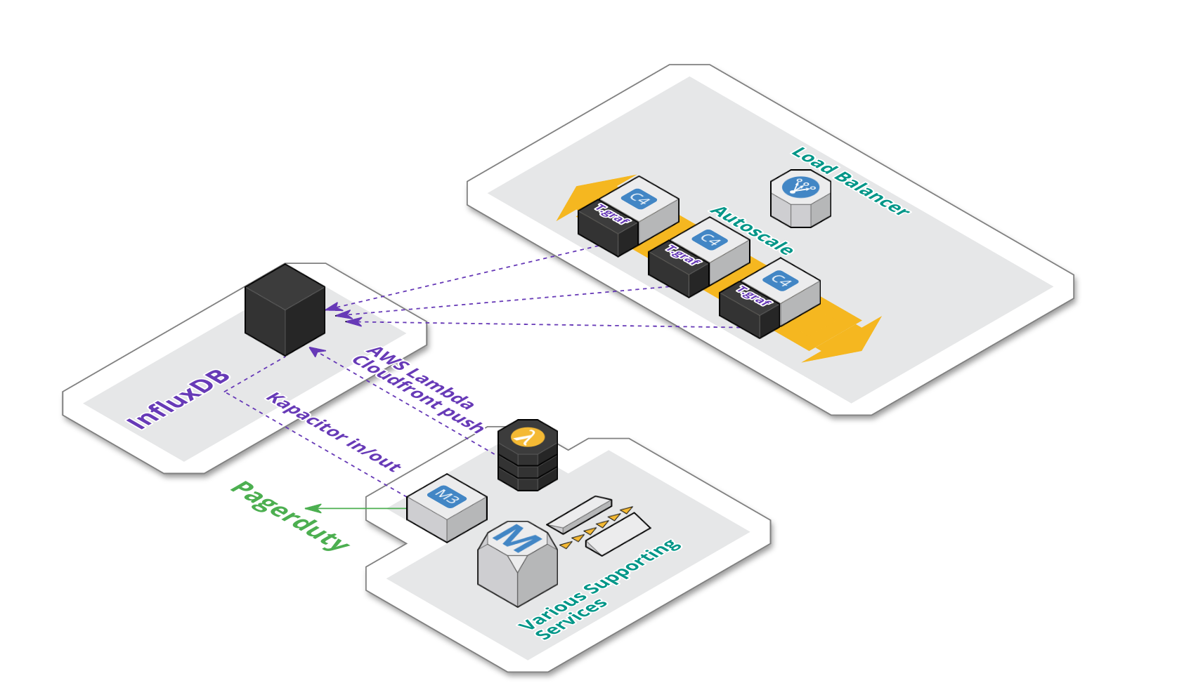
Architecture

Architecturally, our setup remained fairly unchanged. As seen on the schema below:

• We’re currently using a managed instance of InfluxDB provided by influxdata.com.

• Each application server in the auto-scale group still contains an instance of telegraf agent, that aggregate metrics locally and push them to InfluxDB.

• As mentioned, AWS CloudFront metrics are pushed periodically via AWS Lambda.

• We also have an additional dedicated backend EC2 instance for Kapacitor. Kapacitor is responsible for materializing composite metrics. The same component is also responsible for triggering alerts on pagerduty.

Metric based Alerting and Composite Metrics

InfluxDB does not have support for implicit composite metrics. Meaning that you’ll not be able to capture 2 metrics, say request throughput and # of cores in a production cluster and then compute avg request throughput per core. On it’s own, InfluxDB will also not be able to invoke an alert based on a metric threshold.

The InfluxDB stack uses Kapacitor (i.e. InfluxDB data processing platform) to solve both problems of triggering alerts and materializing composite metrics back to InfluxDB using either stream or batch mode for metric processing.

Internally Kapacitor uses a data flow based programming model, where data manipulation nodes can be arranged in a directed acyclic graph. You define such DAG via an surprisingly expressive domain specific language — TICKscript.

Grafana

When we hooked up Grafana to InfluxDB, the whole transition to the TIGK stack started making a lot of sense. We were able to create really expressive dashboards that provide actionable insights into our real time data.

For us it is really valuable to be able to draw out OK and ALERT thresholds explicitly on the dashboard itself and then inline that with either drilldown links or inline markdown documentation — all great core Grafana features.

Grafana and InfluxDB tags

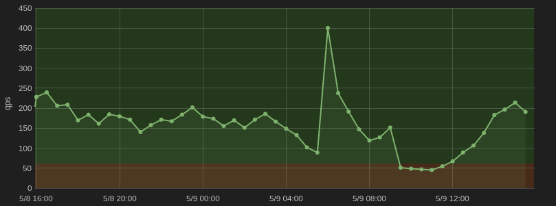
For us, tags became a powerful asset in combination with Grafana templates, since we were able to repeat predefined panels for every tag value in a manner of clicks.

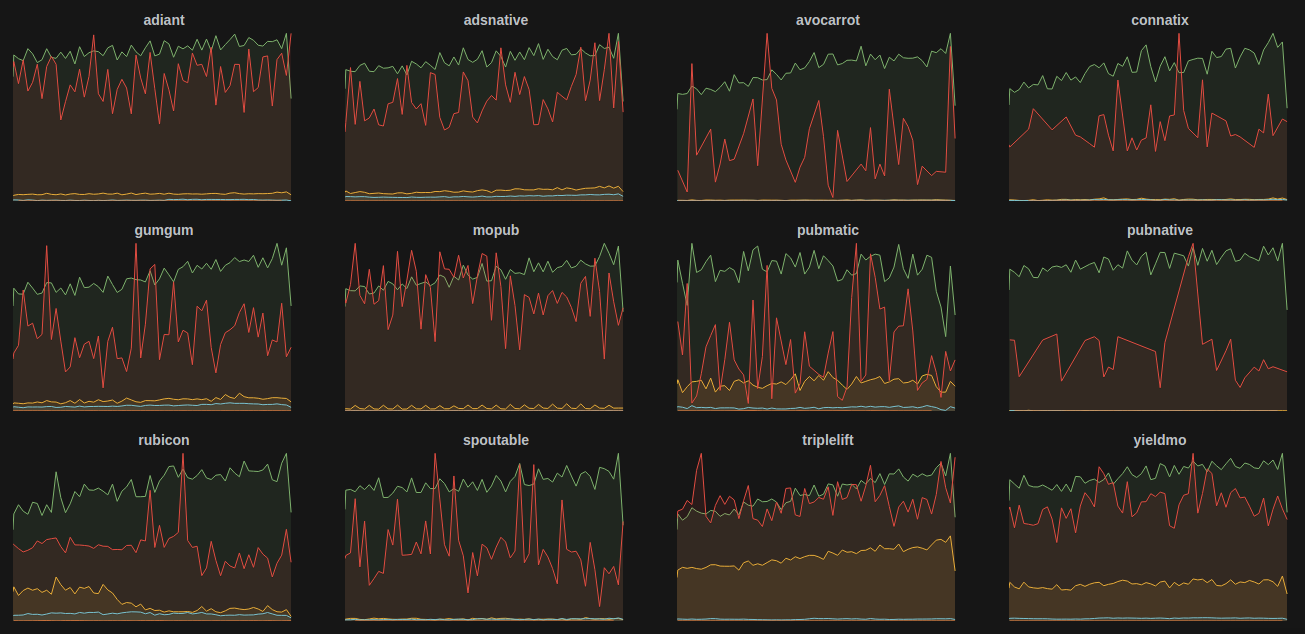
As you can see above, we have a custom tag named exchange (our advertising supply partners) and a couple of metrics we’d like to follow separately for each exchange.

Conclusion

Looking back on our roadmap, from a humble librato beginning, to a more elaborate metric backend stack, we’ve come quite a long way and gathered plenty of experience.

We still have some work on our plates given the current state of affairs, since we’ll soon have to migrate our current managed InfluxDB instance to either the new cloud.influxdata.com offering (we’re currently still on their legacy managed service plan) or migrate to a self-managed version on EC2.

After that we just have to remain focused on nurturing the now freshly created dashboards and make sure only insightful and actionable metrics end up in Grafana.

Discuss this post on Hackers News