Detecting Suspicious Websites

by Aleksandar Dimitriev · 17 Aug 2017

It’s every advertiser’s worst nightmare: advertising on a seemingly legitimate site only to realize that the traffic and/or clicks from that site are not the coveted genuine human interest in the ad. Instead they find fake clicks, unintentional traffic or just plain bots. In a never-ending quest for more ad revenue, some website publishers scramble for ways to increase traffic. And not all approaches are as respectable as improving them site’s content, its readability and SEO.

Some publishers try to boost their stats by buying cheap traffic. Unfortunately, such traffic is often of bad quality. Many sellers that purport to drive good traffic to a site at a extremely small cost actually use botnets to create that traffic.

Botnets can often be detected by looking at which sites share a common set of visitors. Of course, almost all websites share some of their visitors, but this percentage is small. Moreover, as the site accumulates more visitors, the probability of a large overlap occurring by chance becomes infinitesimal. To make things harder a botnet can, among the suspicious sites, visit several well-known and respected websites, so that the apparent credibility of the malicious sites is artificially boosted.

The key is that these botnets re-use the same machines for different “customers”, which we may be able to leverage. The question is thus, can we identify websites infested with such traffic? And if so, then how? The answer to the first question is yes, and to the second is this blog post.

Covisitation graphs

Our problem lends itself nicely to a network approach called a covisitation graph. We will construct a graph, such that the sites that share traffic will be tightly connected. Especially if visitors are shared between several sites, as is usually the case. We can represent all of the websites as vertices (nodes) in a graph. To encode the overlap between a pair or sites, we will use directed edges weighted between 0 and 1. This number will be the proportion of visitors from the source of the edge that were also seen on the target edge. An example is shown in Fig 1. Let A have 200 visitors, B have 1000 visitors, and the shared traffic be 100 visitors. The edge from A to B is the overlap divided by A’s visitors, or 100/200 or 0.5. Similarly, from B to A we have 100/1000 or 0.1. Of course, a network is no network if it’s completely connected. We must set an appropriate threshold to remove edges but keep the ones that are important. A simple threshold of 0.5 proved most useful in our case.

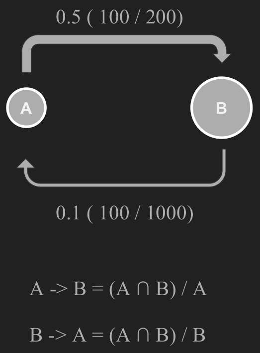Fig. 1. Covisitation edge calculation example.

Clustering coefficient

To get the full network, we must repeat this calculation for all pairs of edges. This network is useful for more than just computation, as a quick visual inspection reveals many interesting things. Tight clusters of websites that are only loosely connected to the core of the graph are precisely the aberrations we would expect when several sites band together. In graph theory, they are called cliques, and have been well researched. A well-known measure of “cliqueness” is the clustering coefficient, shown in Fig. 2.

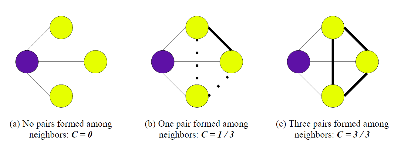Fig. 2. A visual representation of the clustering coefficient. Image courtesy of Santillan et al.

It is a number between 0 and 1, with 0 meaning that none of the node’s neighbors are connected with each other, and 1 meaning the opposite (i.e. the node and its neighbors form a clique). We can combine this number with the probability of such a cluster occurring randomly to get a sensible measure of suspicion for each site. Thus, a small clique of 2-3 sites is somewhat likely to occur, but a clique of 20 nodes warrants a closer discerning look.

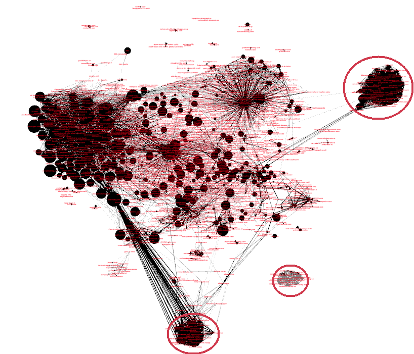Fig. 3. Covisitation graph of all websites with at least 100 unique visitors over a 3-day span. Node size logarithmically proportional to number of visitors.

Results

The circled areas in Fig. 3 indicate exactly these occurrences. We have several groups of websites with dissimilar content where they all share each other’s traffic. One of the suspicious cliques is completely detached from the rest of the graph.

On one hand, there are going to be a lot of naturally occurring edges in the graph. Overlaps as high as 50% are not uncommon between websites of similar content and audience. On the other hand, sites should have very few outgoing edges, especially if they are popular and have many visitors. Popular sites may have many incoming edges, but as long the sources of these edges are not connected with each other it is not suspicious.

Thus, out of the vast interconnected graph that is the world wide web, we can, with precision, pick out the few bad apples that are trying to rake in revenue unfairly and at the detriment of everyone else. We mark such sites as suspicious. This list is then used to avoid buying impressions from these sites and analysing the sources of this traffic. The whole approach outlined in this blog post is one of the tools in Zemanta’s arsenal for combating invalid traffic, where the focus lies in bringing quality traffic for the best possible price.

The analysis was part of my 3-month internship at Zemanta, where I worked on detecting this type of suspicious traffic at scale. The work I’ve done was a breeze with such awesome support from the whole team. It was a great learning experience and an invaluable opportunity to work on a codebase that scales to so many requests per second. Personally, I believe that this bridging of the gap between research and industry benefits both parties immensely, and I hope to do more such collaborations in the future.

Further reading

The original covisitation approach was first used in:

Stitelman, Ori, et al. “Using co-visitation networks for detecting large scale online display advertising exchange fraud.” Proceedings of the 19th ACM SIGKDD international conference on Knowledge discovery and data mining. ACM, 2013,

where our more inquisitive readers can find additional information about this approach.