First steps with Amazon Redshift
by Gregor Ratajc · 13 Mar 2017At Zemanta we have been using Amazon Redshift as our database of choice for campaign traffic statistics. We strive to deliver query results for our analytics view to our users close to real-time. This view is one of the core screens that our users use to manage their campaigns and see how well they perform, so it needs to be in shape.
Amazon Redshift is a great piece of technology but it does not magically produce good results. In fact, performance between an ad-hoc design and an optimized one can differ greatly. Table design and queries that you want to execute need to be tailored to how its internals work best and nourished along the way, when new features get developed and data grows in size. Only then we can get satisfactory results.
In this article we try to sum up the basics of efficient Amazon Redshift table design, and provide some resources that got us going in the right direction.
The basics
Amazon Redshift is a managed data warehousing solution whose main promise is that it can offer fast analytical queries on big data through extensive use of parallelism. It can load and unload big chunks of data directly from or to Amazon S3 (or other AWS storages) with which it integrates seamlessly. This is a big plus if your infrastructure resides in the AWS cloud as ours does. It can effectively do large data transformations and so can be used for your ELT (Extract, load, transform) pipeline. This is a great article from Panoply that compares ELT and ETL - the more common way of transforming data before loading it.
One of the common first impressions is that it’s actually some kind of PostgreSQL database because you can communicate with it with tools that are made for PostgreSQL, e.g. psql. It actually emerged from it, but as we will see, it is really far from it and should be treated differently.
Cluster
When you start using Redshift, you provision a cluster. A cluster consists of a leader node and multiple compute nodes. These are further subdivided into slices.
The leader receives queries, optimizes them, creates query plans and coordinates the work amongst its nodes. A node provides CPU, memory and disk for query execution and data storage. Memory and storage are proportionally allocated to its slices. A slice executes a single query segment within one process at a time.
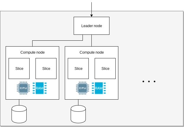 Amazon Redshift cluster arhitecture.
More on cluster arhitecture and query execution workflow can be found in the official documentation here and here.
Data storage
The way data is stored and organized within a cluster directly influences how tables and queries should be designed for them to be performant.
The four most important concepts of data organization are: data distribution, sort keys, zone maps and compression. Here we will cover them briefly and provide some additional resources where you can research them in more depth.
Distribution
Distribution determines how data is distributed among slices. With it we define by what strategy should records be grouped together. By that we put data where it needs to be beforehand and so reduce the need for query optimizer to move data between nodes to efficiently query it. This comes in handy when we join data.
In the following example of data distribution we see traffic and conversion records grouped by campaign. When we join such data by campaign, no records need to be redistributed between nodes as they can be joined within a single slice. If distribution would be different and we would want to make the same join, records would need to be relocated temporarily before a query would execute.
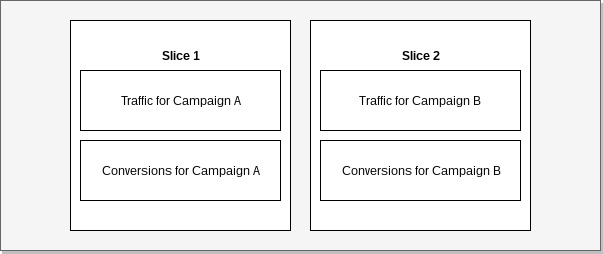 Example: Data collocation.
With a proper distribution strategy we also try to evenly load nodes so that parallel processes have similar amount of work to do. The end processing time is determined by the slowest process. A node that has disproportionate amount of work to do, will thus directly influence the overall query execution time.
The consequence of uneven data grouping is skew (Skewed table data). In such cases some slices contain more data than others and can therefore slow our queries and cause premature fill up of storage on some nodes.
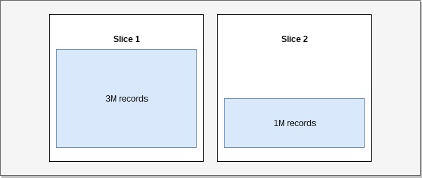 Example: Skew.
Sort keys and zone maps
Redshift stores data in columns. This means that blocks of values from the same column are stored on disk sequentially as opposed to row based systems where values from a row follow sequentially.
Sequential values of a column are partitioned within 1MB blocks that represent the smallest data organizational unit. Redshift will load an entire block to fetch a value from it, so it is important for us to understand how it decides to select a block. This way we can minimize I/O operations.
Sort keys set the order of records within blocks and tables. It
behaves the same as ORDER BY in queries.
Zone maps are meta data about blocks, they define MIN and MAX value within them. Using sort key and zone map information Redshift can skip blocks that are irrelevant for a particular query.
In the following example we will try to illustrate the difference in the amount of I/O required to locate the offset of relevant records. We defined a table that has clicks grouped by date and campaign id. We have ordered the data by date. To query clicks by campaign for the date 2017/02/12, Redshift will be able to find relevant records by loading and reading only the 1st date column block. On the other hand, when we would like to get clicks for campaign id 500, 2 blocks will have to be loaded and read to get the record offset for other columns.
CREATE TABLE stats (
    date date not null,
    campaign_id int2 encode lzo,
    clicks integer encode lzo
) sortkey(date)
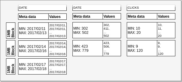 Example: Sort keys and zone maps.
When adding data to our tables we need to maintain the sort and meta data. We can either add
data in correct order or we can use VACUUM to resort and ANALYZE to update meta data
and table statistics.
Compression
Due to Redshifts columnar nature it can efficiently compresses the data it holds. This means that the amount of data within a 1MB block can be increased and the overall storage footprint reduced. This can save us some I/O because less data needs to be read from a disk. Because it is columnar it can also independently of other columns shrink or grow records within one column.
In the Sort keys and zone maps example we can see different storage requirements for the date and campaign id columns. We see that the same amount of values for dates took 3 blocks, and only 2 blocks for campaign ids. This happened because the compression of the campaign column was better.
By default no compression is applied to data. A good first start is the command ANALYZE COMPRESSION
that we execute on already loaded data and it will give us recommended encodings based on a sample. If we have
some knowledge about our data we can also select encodings ourselves. Available algorithms and when to use them
are listed here.
Code compilation
Not related to the way data is stored but important concept used by Amazon Redshift is code compilation.
When Redshift receives a query, it will optimize it and generate a query plan. Execution engine will take that query plan and generate compiled C++ code from it. After that it will put it into a LRU cache. The compilation step can take a while and this is why you will notice that the 1st run of a query is always, sometimes by an order of magnitude, slower than the following runs of the same query. Later runs of the same (or similar) query will take the compiled code from cache and thus the compilation step will be skipped.
A query won’t need to be recompiled if only some filter parameters get changed. On the other hand, Redshift will recompile a query if everything is the same but different or additional columns are selected. Unfortunatelly not much is documented about what changes have an effect on recompilation. In this article the author tries to experiment a bit and find some patterns.
Cases when we need to be aware of this behaviour are benchmarks and dynamic query building. When we do benchmarks we always ditch the first query execution time as it will always be an outlier. Where we do dynamic query building we try to reduce the number of unique queries. One way we do that is that we always query all columns that are available for a given view. We strip the ones that we won’t show later, e.g. based on a permission. This way a query for the same view but two users with different permissions will be the same or similar enough that it won’t need to be recompiled.
Conclusion
We have been using Amazon Redshift for more than a year now and we are pretty comfortable with it by now. We think the concepts described in this article will give you a good start with fundamentals of optimal table design that are needed for a beginner in this field.
We realize there is a lot more to it, so we selected a few more resources that helped us, and we are sure will help you, on going further and deeper on it in the last chapter Additional resources of this article.
Additional resources
- Top 10 Performance Tuning Techniques for Amazon Redshift
- Improving Redshift Query Performance Through Effective Use of Zone Maps
- The Lazy Analyst’s Guide to Amazon Redshift
- The Hitchhiker’s Guide to Redshift
- Amazon Redshift Deep Dive
- Deep Dive: Amazon Redshift for Big Data Analytics (video)
- Redshift at Lightspeed: How to continuously optimize and modify Redshift schemas
- Amazon Redshift - Database Developer Guide (official documentation)